Speeding up Python with Mojo🔥

Speedup Python implementation in Mojo for simple Euclidean distance calculation

In this example we’ll calculate the Euclidean distance between two n-dimensional vectors a and b mathematically expressed as the L2-norm of the difference vector: $$ ||a-b||_2 $$

Let’s start by creating 2 random n-dimensional numpy arrays in python Notice that the cell starts with %%python i.e. this cell will execute in Python, no Mojo. We’ll use this to compare performance between Python and Mojo implementations.

%%python
import time
import numpy as np
from math import sqrt
from timeit import timeit

n = 1000000
np.random.seed(42)
arr1_np = np.random.rand(n)
arr2_np = np.random.rand(n)

arr1_list = arr1_np.tolist()
arr2_list = arr2_np.tolist()

def print_formatter(string, value):
    print(f"{string}: {value}")

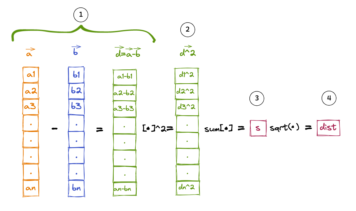
Below is a Python function which takes arr1_list and arr2_list as arguments and calculates the eculidean distance using the following steps:

1. Calculate the element-wise difference between two vectors to create a difference vector
2. Square each element in the difference vector
3. Sum up all the squared elements of the difference vector
4. Take the square root of the sum

Go ahead and run the cell and take a note of the value and duration

%%python
# Pure python iterative implementation
def python_dist(a,b):
    sq_dist = 0.0
    n = len(a)
    for i in range(n):
        diff = a[i]-b[i]
        sq_dist += diff*diff
    return sqrt(sq_dist)

tm = timeit(lambda: python_dist(arr1_list,arr2_list), number=5)/5
print("=== Pure Python Performance ===")
print_formatter("value", python_dist(arr1_list,arr2_list))
print_formatter("time (ms)", 1000*tm)

Let’s compare pure-Python performance with NumPy. NumPy takes advantage of optimized linear algebra subroutines to accelerate these calculations. Run the cell below and take a note of the speedup.

%%python
def python_numpy_dist(a,b):
    return np.linalg.norm(a-b)

tm = timeit(lambda: python_numpy_dist(arr1_np,arr2_np), number=5)/5
print("=== NumPy Performance ===")
print_formatter("value", python_numpy_dist(arr1_np,arr2_np))
print_formatter("time (ms)", 1000*tm)

Time to Mojo🔥! Run the following cell to copy over the numpy arrays from Python to Mojo🔥 tensors so can compare not only the execution time but also verify the accuracy of the calculations.

from tensor import Tensor
from time import now
from math import sqrt

let n: Int = 1000000
alias dtype = DType.float64
var arr1_tensor = Tensor[dtype](n)
var arr2_tensor = Tensor[dtype](n)

for i in range(n):
    arr1_tensor[i] = arr1_np[i].to_float64()
    arr2_tensor[i] = arr2_np[i].to_float64()

Exercise: Copy over the pure-Python function into Mojo🔥 and variable declaration and return types, you did in notebook 1.

fn mojo_dist(a: Tensor[dtype], b: Tensor[dtype]) -> Float64:
    var sq_dist:Float64 = 0.0
    let n = a.num_elements()
    for i in range(n):
        let diff = a[i]-b[i]
        sq_dist += diff*diff
    return sqrt(sq_dist)

#Hint: Insert function below with the following signature
#fn mojo_dist(a: Tensor[dtype], b: Tensor[dtype]) -> Float64: ...

Copy paste the following the same cell to benchmark

let eval_begin = now()
let mojo_arr_sum = mojo_dist(arr1_tensor,arr2_tensor)
let eval_end = now()

print("=== Mojo Performance ===")
print_formatter("value", mojo_arr_sum)
print_formatter("time (ms)", Float64((eval_end - eval_begin)) / 1e6)

Accelerating Mojo🔥 code with Vectorization

Modern CPU cores have dedicated vector register that can perform calculations simultaneously on fixed length vector data. For example an Intel CPU with AVX 512 has 512-bit vector register, therefore we have 512/64=8 Float64 elements on which we can simultaneously perform calculations. This is referred to as SIMD = Single Instruction Multiple Data. The theoretical speed up is 8x but in practice it’ll be lower due to memory reads/writes latency.

Note: SIMD is should not be confused with parallel processing with multiple cores/threads. Each core has dedicated SIMD vector units and we can take advantage of both SIMD and parallel processing to see massive speedup as you’ll see in notebook 3

First, let’s gather the simd_width for specific dtype on the specific CPU you’ll be running this on.

from sys.info import simdwidthof
from algorithm import vectorize
alias simd_width = simdwidthof[DType.float64]()

To vectorize our naive mojo_dist function, we’ll write a closure that is parameterized on simd_width. Rather than operate on individual elements, we’ll work with simd_width elements which gives us speed ups. You can access simd_width elements using simd_load.

Given that this is a complex topic, I’ve provided the solution below, please raise your hand and ask the instructor for explainations if anything is unclear.

fn mojo_dist_vectorized(a: Tensor[DType.float64], b: Tensor[DType.float64]) -> Float64:
    var sq_dist: Float64 = 0.0
    @parameter
    fn simd_norm[simd_width:Int](idx:Int):
        let diff = a.simd_load[simd_width](idx) - b.simd_load[simd_width](idx)
        sq_dist += (diff*diff).reduce_add()
    vectorize[simd_width, simd_norm](a.num_elements())
    return sqrt(sq_dist)

let eval_begin = now()
let mojo_arr_vec_sum = mojo_dist_vectorized(arr1_tensor,arr2_tensor)
let eval_end = now()

print_formatter("value", mojo_arr_vec_sum)
print_formatter("time (ms)",((eval_end - eval_begin)) / 1e6)